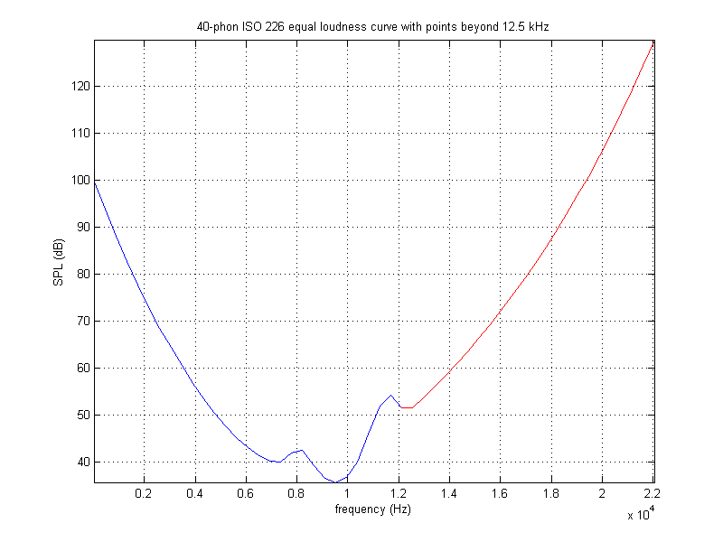


This time, apply an equal loudness contour by filtering in the frequency domain.
With code heavily borrowed from Dr. Scordilis' ideal_filtering_ola.m, the filtering process goes like this:
function [filename] = project_03_part02def(filename)
%filename = 'invisible.wav';
close all;

[signal,fs] = wavread(filename);
%signal = randn(fs*5,1);
signal = signal';
t = 0:1/fs:(length(signal)-1)/fs;
figure(1), subplot(211), plot(t, signal,'Color',[0.6666, 0.8235, 1]), grid on, axis tight;
title(['input signal (',filename,')']), xlabel('time (s)'), ylabel('amplitude');
%soundsc(signal, fs);

%-- PLOTTING SECTION for positive frequencies of FFT ----------------------
%number of pts for FFT, length of signal should be default. use more points
%for higher frequency resolution
n_fft_points = length(signal)*5;
signal_fft = fft(signal,n_fft_points);
T = n_fft_points/fs;                    %get frequency interval
freq = (0:n_fft_points-1)/T;            %create frequency range
%only want first half of the FFT, since it is mirrored and redundant
cutoff = ceil(n_fft_points/2);
freq = freq(1:cutoff);
signal_freq_positive = signal_fft(1:cutoff);
signal_freq_positive = signal_freq_positive/max(signal_freq_positive); %normalize the data

figure(2), subplot(211), plot(freq,abs(signal_freq_positive),'Color',[0.9490,0.7451,0.0510]), grid on, axis tight;
%axis([0,fs/3,0,1]);
title(['FFT of input signal (',filename,'), N=',num2str(n_fft_points)]), xlabel('frequency (Hz)'), ylabel('amplitude');

figure(3), plot(freq,abs(signal_freq_positive),'Color',[0.9490,0.7451,0.0510]), grid on, axis tight;
%axis([0,fs/3,0,1]);
title(['FFT of input signal (',filename,'), N=',num2str(n_fft_points)]), xlabel('frequency (Hz)'), ylabel('amplitude');
print project_03_part02d_input_large_fft -dpng -r100;

%-- generate equal loudness curve -----------------------------------------
equal_loudness_curve = iso226(40);      %original Fletcher-Munson curve was at 40-phon
orig_elc_freq_min = 20;                 %ISO 226 starts at to 20 Hz
orig_elc_freq_max = 12500;              %ISO 226 goes up to 12.5 kHz
orig_elc_data_pts = 29;                 %ISO 226 gives 29 frequency points
orig_elc_length = length(equal_loudness_curve);
extra_pts = 0;
if(orig_elc_freq_max < fs/2)
    extra_pts = ceil(orig_elc_data_pts*(fs/2)/orig_elc_freq_max) - orig_elc_data_pts;
    extra_values = logspace(log(equal_loudness_curve(length(equal_loudness_curve)))/log(10),...
        log(1.3*max(equal_loudness_curve))/log(10),extra_pts);
    equal_loudness_curve = [equal_loudness_curve,extra_values];
end

f = linspace(orig_elc_freq_min,fs/2,orig_elc_data_pts+extra_pts);
figure(4), plot(f,equal_loudness_curve,'b',f(orig_elc_length:length(equal_loudness_curve)),...
    equal_loudness_curve(orig_elc_length:length(equal_loudness_curve)),'r'), grid on, axis tight;
title('40-phon ISO 226 equal loudness curve with points beyond 12.5 kHz'), xlabel('frequency (Hz)'), ylabel('SPL (dB)');
print project_03_part02e -dpng -r100;

%% ANALYSIS/RESYNTHESIS USING THE OVERLAP-ADD METHOD
time_window = 25e-3;
%analysis window size should be power of 2
window_size = 2^nextpow2(round(time_window*fs));
window = hamming(window_size)';         %window function type
window_shift = window_size/4;           %amount to shift window for overlap-add
%initialize by appending zeros
signal = [zeros(1,window_size) signal zeros(1,window_size)];
new_signal = zeros(1,length(signal)+4*window_size);
frame = zeros(1,window_size);           %initialize frame

print_fig_5 = false;
for i=1:window_shift:length(signal)-window_size
    frame = signal(i:i+window_size-1);	%select analysis frame
    frame = frame.*window;              %apply window function
    %appending zeros at both ends of frame gives best frequency resolution during FFT
    frame = [zeros(1,window_size) frame zeros(1,window_size)];

    %number of pts for FFT, length of signal should be default. use more points
    %for higher frequency resolution
    n_fft_points = length(frame);
    frame_freq_domain = fft(frame,n_fft_points);
%%{
    %-- PLOTTING SECTION for positive frequencies of FFT ------------------
    T = n_fft_points/fs;                %get frequency interval
    freq = (0:n_fft_points-1)/T;        %create frequency range
    %only want first half of the FFT, since it is mirrored and redundant
    cutoff = ceil(n_fft_points/2);
    freq = freq(1:cutoff);
    frame_freq_positive = frame_freq_domain(1:cutoff);
    frame_freq_positive = frame_freq_positive/max(frame_freq_positive); %normalize the data

    figure(5), subplot(211), plot(freq,abs(frame_freq_positive),'Color',[0.9490,0.7451,0.0510]), grid on, axis tight;
    %axis([0,fs/3,0,1]);
    %axis([fs/4,fs/2,0,1]);
    title(['analysis frame before filtering, N=',num2str(n_fft_points)]), xlabel('frequency (Hz)'), ylabel('amplitude');
    print_fig_5 = true;
 %}
    %-- FILTERING SECTION -------------------------------------------------
%%{
    %-- EQUAL LOUDNESS-----------------------------------------------------
    elc_interp = spline(0:length(equal_loudness_curve)-1,equal_loudness_curve,...
        0:length(equal_loudness_curve)/(length(frame_freq_domain)/2-1):length(equal_loudness_curve));

    frame_freq_domain(1:length(frame_freq_domain)/2) = elc_interp.*frame_freq_domain(1:length(frame_freq_domain)/2);
    frame_freq_domain(length(frame_freq_domain)/2+1:length(frame_freq_domain)) = fliplr(elc_interp).*frame_freq_domain(length(frame_freq_domain)/2+1:length(frame_freq_domain));
%}
%%{
    %-- PLOTTING SECTION for positive frequencies of FFT ------------------
    T = n_fft_points/fs;                %get the frequency interval
    freq = (0:n_fft_points-1)/T;        %create frequency range
    %only want first half of the FFT, since it is mirrored and redundant
    cutoff = ceil(n_fft_points/2);
    freq = freq(1:cutoff);
    frame_freq_positive = frame_freq_domain(1:cutoff);
    frame_freq_positive = frame_freq_positive/max(frame_freq_positive); %normalize the data

    figure(5), subplot(212), plot(freq,abs(frame_freq_positive),'Color',[0.9490,0.7451,0.0510]), grid on, axis tight;
    %axis([0,fs/3,0,1]);
    %axis([fs/4,fs/2,0,1]);
    title(['analysis frame after filtering, N=',num2str(n_fft_points)]), xlabel('frequency (Hz)'), ylabel('amplitude');
    print_fig_5 = true;
 %}
     print project_03_part02f_filtering -dpng -r100;
    %-- SIGNAL RECONSTRUCTION with overlap-add ----------------------------
    frame_time_domain = (window_shift/window_size)*real(ifft(frame_freq_domain));
    new_signal(i:i+length(frame)-1) = new_signal(i:i+length(frame)-1) + frame_time_domain;
    %pause(0.1)         %for visualization of graph changes in slow motion
end

if(print_fig_5)
    print project_03_part02f_filtering -dpng -r100;
end

new_signal = new_signal./max(abs(new_signal));         %normalized signal
t = 0:1/fs:(length(new_signal)-1)/fs;
figure(1), subplot(212), plot(t,new_signal,'Color',[0.6666, 0.8235, 1]), grid on, axis tight;
title(['filtered signal (',filename,')']), xlabel('time (s)'), ylabel('amplitude');
print project_03_part02df_signal -dpng -r100;

%-- PLOTTING SECTION for positive frequencies of FFT ----------------------
n_fft_points = length(new_signal)*5;
new_signal_fft = fft(new_signal,n_fft_points);
T = n_fft_points/fs;                    %get frequency interval
freq = (0:n_fft_points-1)/T;            %create frequency range
%only want first half of the FFT, since it is mirrored and redundant
cutoff = ceil(n_fft_points/2);
freq = freq(1:cutoff);
new_signal_freq_positive = new_signal_fft(1:cutoff);
new_signal_freq_positive = new_signal_freq_positive/max(new_signal_freq_positive); %normalize the data

figure(2), subplot(212), plot(freq,abs(new_signal_freq_positive),'Color',[0.9490,0.7451,0.0510]), grid on, axis tight;
%axis([0,fs/3,0,1]);
title(['FFT of filtered signal (',filename,'), N=',num2str(n_fft_points)]), xlabel('frequency (Hz)'), ylabel('amplitude');
print project_03_part02df_fft -dpng -r100;

figure(6), plot(freq,abs(new_signal_freq_positive),'Color',[0.9490,0.7451,0.0510]), grid on, axis tight;
%axis([0,fs/3,0,1]);
title(['FFT of filtered signal (',filename,'), N=',num2str(n_fft_points)]), xlabel('frequency (Hz)'), ylabel('amplitude');
print project_03_part02f_output_large_fft -dpng -r100;

soundsc(new_signal, fs);
wavwrite(new_signal,fs,'project_03_part02f');
|
 |
 |
 |
 |
 |
 |