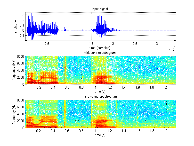
Speak your name (first and last) continuously and create a digital version of it using sampling rate of fs = 16 kHz and 16 bit linear quantization. Plot the time waveform, wideband spectrogram, and narrowband spectrogram.
Here, all that needed to be done was to apply pre-defined parameters for wideband and narrow spectrograms into code.
function project_03_part01abc()

[signal,fs,nbits] = wavread('eliot_peng.wav');

subplot(311), plot(signal), grid on, axis tight;
title('input signal'), xlabel('time (samples)'), ylabel('amplitude');

f = linspace(0,8000,500);

%C) Narrowband Spectrogram
%Window type: Hamming
%Window size: 20 to 25 ms
%Window overlap: 97%
nb_window_size = round(0.0225*fs);
nb_window_overlap = round(nb_window_size*0.97);
subplot(313), spectrogram(signal,nb_window_size,nb_window_overlap,f,fs,'yaxis'), grid on, axis tight;
title('narrowband spectrogram'), xlabel('time (s)'), ylabel('frequency (Hz)');

%B) Wideband Spectrogram
%Window type: Hamming
%Window size: 1/4 of narrowband case
%Window overlap: 90%
wb_window_size = round(nb_window_size/4);
wb_window_overlap = round(wb_window_size*0.90);
subplot(312), spectrogram(signal,wb_window_size,wb_window_overlap,f,fs,'yaxis'), grid on, axis tight;
title('wideband spectrogram'), xlabel('time (s)'), ylabel('frequency (Hz)');

%soundsc(signal,fs);
%print project_03_part01_r100 -dpng -r100;
%print project_03_part01_r150 -dpng -r150;
|
|