function [signal] = project_01_part02(f0, fs, secs, velocity, dist_from_track)

%comment out f0, fs, secs, velocity, and dist_from_track to specify values
%from command line
c = 340;                %speed of sound
velocity = 10;          %velocity of sound source
f0 = 440;               %center frequency of sound
fs = 8000;              %sampling frequency
secs = 10;              %duration of sound
dist_from_track = 5;    %shortest distance from observer to track

time = -secs/2:1/fs:secs/2;
x = velocity*time;      %x-position of sound source on track

hypo = zeros(1,length(time));
%change in hypotenuse equals relative distance from sound source to observer
for i = 1:length(hypo)
    hypo(i) = sqrt((x(i))^2 + dist_from_track^2);
end

env = 1./hypo;
%velocity relative to observer is orig velocity vector * adj/hypo (cosine)
vel_rel_observer = velocity*x./hypo;

f = zeros(1,length(time));
for i = 1:length(time)
    f(i) = f0*(c/(c+vel_rel_observer(i)));
end

signal = env.*sin(2*pi*f.*time);

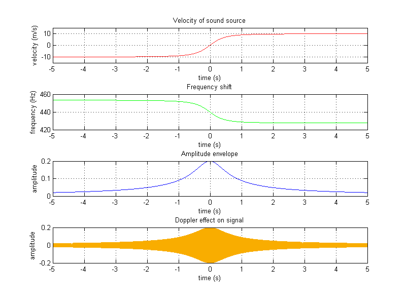
subplot(411), plot(time,vel_rel_observer,'Color',[1,0.12,0.12]), axis([min(time),max(time),-1.5*velocity,1.5*velocity]), grid on;
title('Velocity of sound source'), xlabel('time (s)'), ylabel('velocity (m/s)');
subplot(412), plot(time,f,'g'), grid on;
title('Frequency shift'), xlabel('time (s)'), ylabel('frequency (Hz)');
subplot(413), plot(time,env,'b'), grid on;
title('Amplitude envelope'), xlabel('time (s)'), ylabel('amplitude');
subplot(414), plot(time,signal,'Color',[0.98,.68,0]), grid on;
title('Doppler effect on signal'), xlabel('time (s)'), ylabel('amplitude');

signal = signal/max(abs(signal)); %normalizes input

%print project_01_part02 -dpng -r100;
%wavwrite(signal,fs,'project_01_part02');

soundsc(signal,fs);