Speak your name (first and last) continuously and create a digital version of it using sampling rate of fs = 16 kHz and 16 bit linear quantization. In a single figure window:

      

        a. Plot the time waveform.

        b. Plot the wideband spectrogram.

        c. Plot the narrowband spectrogram.

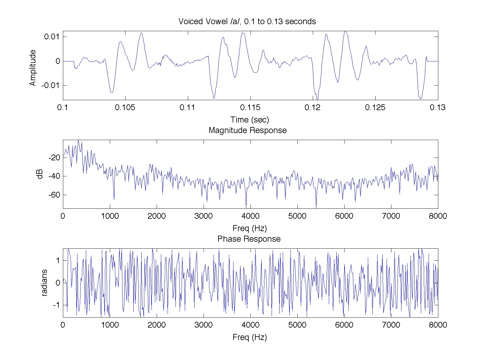
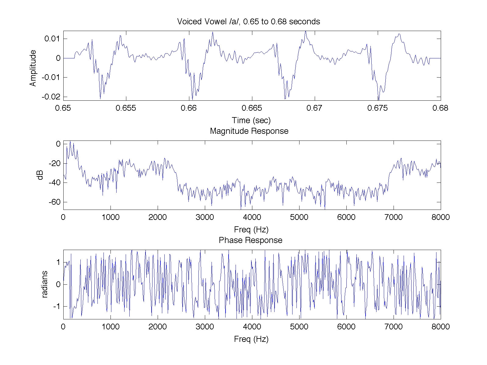
        d. Select two different 30 ms vowel segments in the recorded utterance and plot their magnitude (dB vs. Hz) and phase spectra (radius vs. Hz) spectra, from 0 Hz to fs/2 Hz.

________________________________________________________________________

        In section 1, I was required to digitally record myself speaking my first and last name continuously with a bit depth (bd) of 16 bits and a sampling rate (fs) of 16 kHz.  In digital recording, bd is the number of bits allotted to store the amplitude of each sample.  fs determines how often snap shots, called samples, are taken from the continuous analog input signal.  fs = 1 / T, where T is the period of time between samples.

        In sampling theory, only frequencies below half the sampling frequency, fs / 2, can be accurately captured. Therefore, in the case of fs = 16 kHz, only frequencies between 0 and 8000 Hz can be recorded. For analyzing the human voice, this frequency range is adequate because the majority of human speech frequencies lies in this range.        

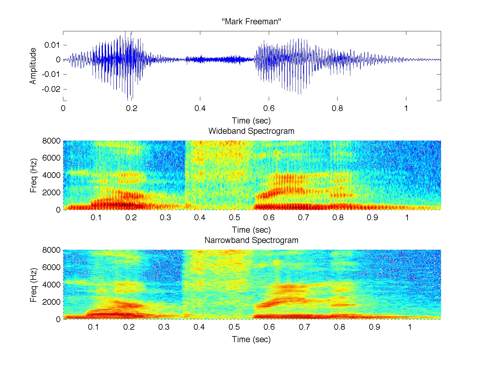
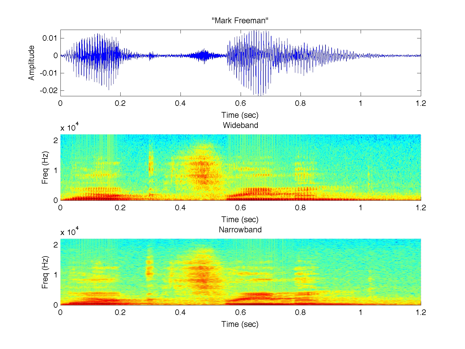
        I wanted to be able to analyze my voice in the full range of human hearing, from 20 to 20 kHz.  So I sampled my voice twice, first at the required fs = 16 kHz and then at fs = 44.1 kHz.  I graphed the plots for a., b., and c. with the fs = 16 kHz  recording in Figure 1.1 using MATLAB’s spectrogram function.  I then tried to plot a., b., and c. with the fs = 44.1 kHz recording, but it seems that the MATLAB spectrogram function can only plot recordings with sampling rates less than or equal to 16 kHz.

     

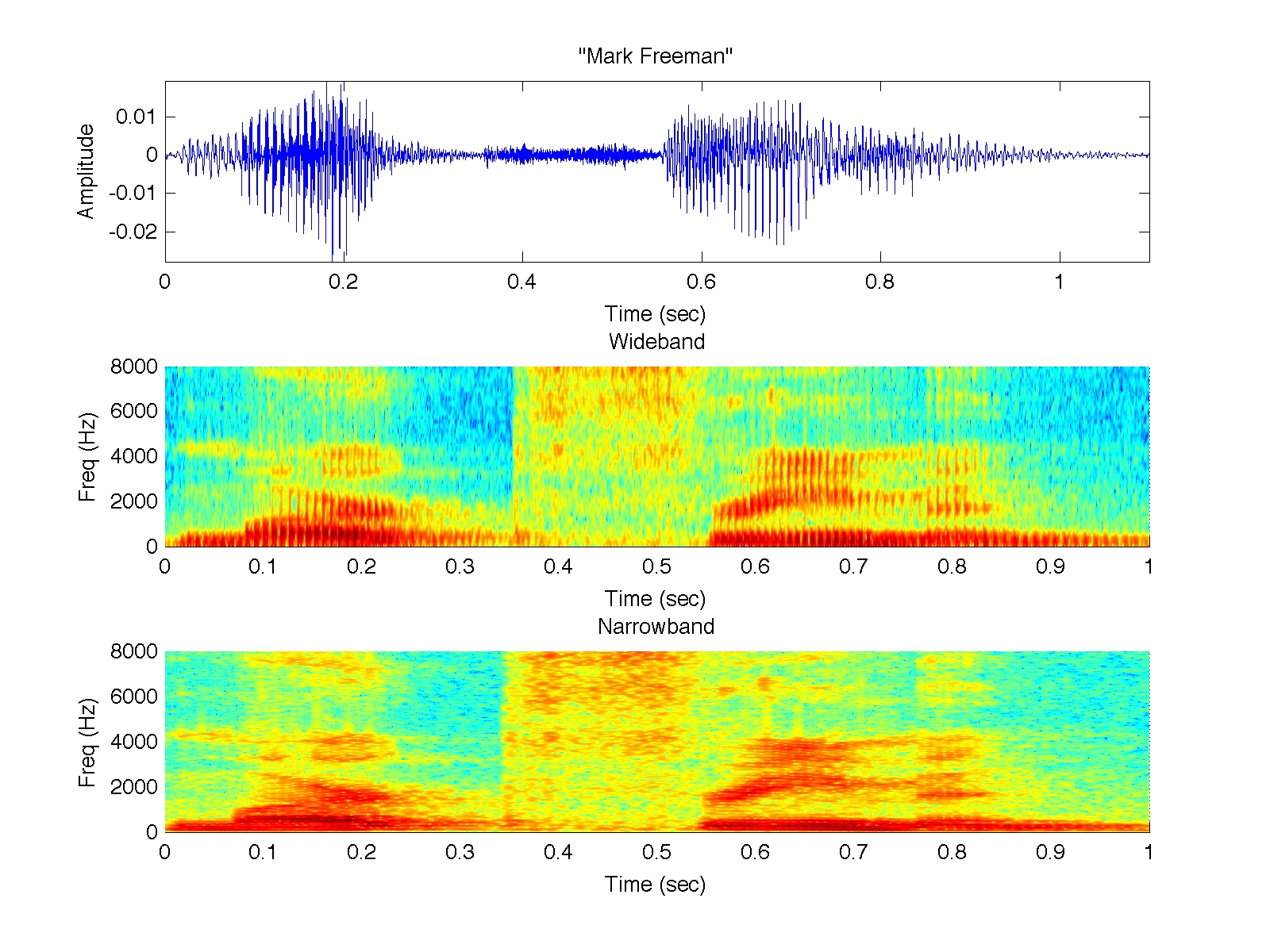
      I was frustrated with this discovery and so I decided to write my own spectrogram function in MATLAB.  To read about how I did this and to see the MATLAB code, click here.  Figure 1.2 shows the fs = 16 kHz recording plotted with my spectrogram function.  Figure 1.3 shows the fs = 44.1 kHz recording plotted with my spectrogram function.

________________________________________________________________________

Parts a. through c.       View MATLAB CODE for a, b, and c here.

Figure 1.1.   Shows the recording of me speaking my first and last name using

                    MATLAB’s spectrogram function at fs = 16 kHz.  

                    a. (top), Amplitude vs Time.

                    b. (middle), Wideband Spectrogram.

                    c. (bottom), Narrowband Spectrogram.

-------------------------------------------------------------------------------------------------------------

Figure 1.2.   Shows the recording of me speaking my first and last name using

                    my spectrogram function at fs = 16 kHz.  

                    a. (top), Amplitude vs Time.

                    b. (middle), Wideband Spectrogram.

                    c. (bottom), Narrowband Spectrogram.

-------------------------------------------------------------------------------------------------------------

Figure 1.3.   Shows the recording of me speaking my first and last name using

                    my spectrogram function at fs = 44.1 kHz.  

                    a. (top), Amplitude vs Time.

                    b. (middle), Wideband Spectrogram.

                    c. (bottom), Narrowband Spectrogram.

________________________________________________________________________

Part d.                View MATLAB Code for d here

Back